Profiling and Film Emulation Overview.

For ones that are not familiar with the scientific approach to film emulation here’s a quick overview to understand what we’ll be covered in the coming lessons. The concept is the following. In order to create an accurate profile/emulation of a film stock we need to capture a lot of colors (stimuli) with a digital camera and the film stock we want to emulate, side by side under the same exact conditions all across the exposure range. The scope is to have an accurate comparison of how the digital sensor and the film stock respond to light. To do this we’re going to use color charts and capture thousands of color samples. Once the negative or the print (if we’re going for a print profile) is scanned, the RGB values of the color charts are then measured and saved to text files that represent the 2 datasets (digital and film). The 2 text files containing the datasets are then fed to a Color Matching Algorithm that will output a color transformation to match digital to film.

The precision of the transformation is influenced by the quality of the datasets. You’ll see how creating a robust dataset is not trivial and there many things to keep in mind to get accurate results. Those are gonna be covered in detail in the coming lessons but here’s a quick introduction

The color stimuli produced by an object and illuminated by a light source can be measured with spectrometer and plotted on the 1931 CIE graph. The 1931 CIE graph gives us a visual representation of the visible spectrum (the spectrum of light that humans can see). The image below shows the plot of the color patches of a Color Checker Classic illuminated by D50 illuminant (daylight).

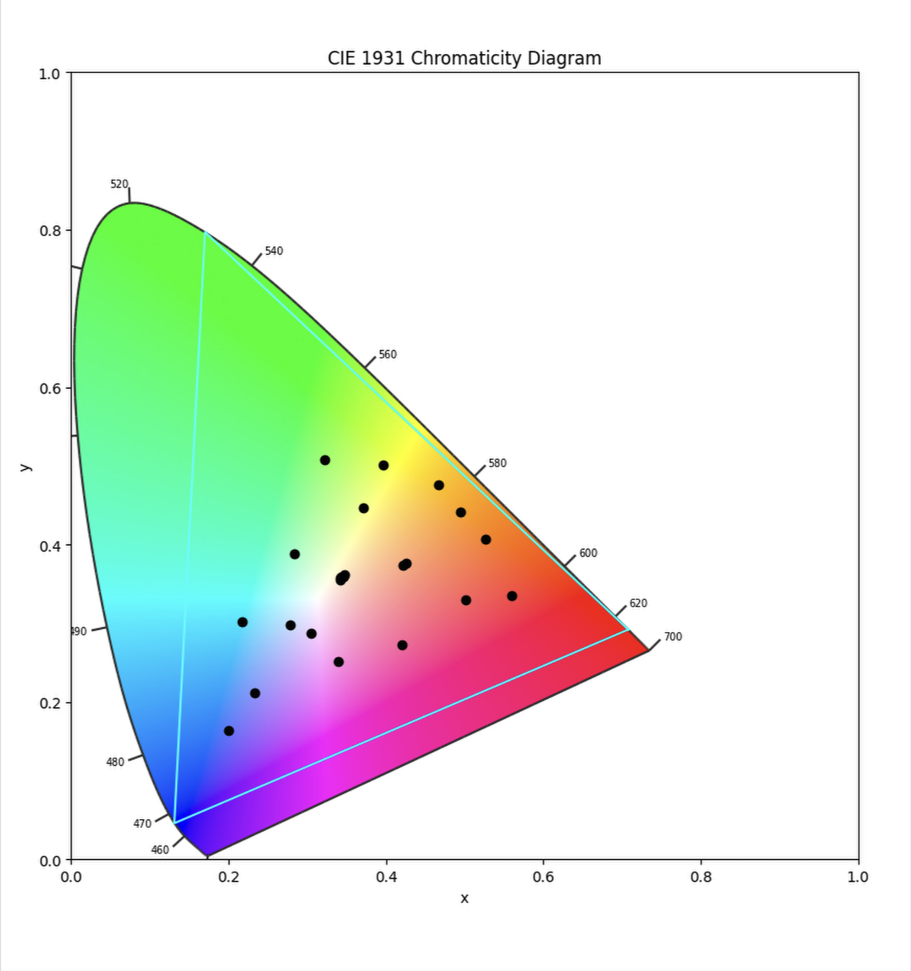
In the image above: This is what most folks do when creating a dataset for their film emulation by shooting a Color Checker Classic under one illuminant. It should be clear that, in this scenario, even if we match a few data points (like these ones in the color checker classic), it’s not possible to create a profile that works in any scenario and illumination simply because the dataset is too limited and it doesn’t allow us, nor a matching algorithm to know how a color that lies outside those few datapoints should be rendered.

What we’re going to be doing instead

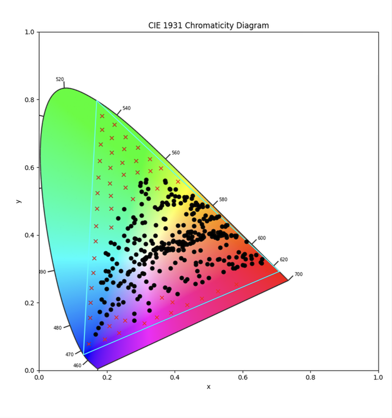
In the image above: This is the dataset we will be creating by following the workflow and techniques discussed in the following lessons. The dotted points are the plots of the reflective charts used (Color checker classic + Color checker SG under 3 different illuminants) while the X’s are the plots of the emissive high saturation colors (more on that later) It’s a much more comprehensive datasets that allows to create profiles that will be accurate and reliable no matter the lighting condition.

With the workflow described here and with the tools and techniques that that I’ll share with you, you’ll be able to create any type of profile you desire, and be fully in control of the photographic look of your images.

In the coming lessons we’re going to discuss everything from shooting charts, scanning, preparing the datasets for profiling…but you’ll also be provided with charts that I shot so that you can follow along, learn and create high end profiles even if you don’t have the chance to shoot and scan your own charts.

NB: The triangle represent rec2020 gamut, while it is true that we cannot produce and measure all the colors in the visible spectrum as we’re limited by lighting fixture that cannot emit a spectrum of light that is wider gamut than rec2020, it doesn’t seem to me to be necessary as film could not reproduce those colors anyway.

The images below show the subtle—but all the more beautiful—difference between the ARRI Rec.709 color pipeline and a profile of Kodak Ektachrome slide film. Here we don’t have a flashy film look. This is a scientific profile of a positive film stock. The painterliness is all there!