
ADVANCED GRAIN PROFILING AND COMPOSITING
The textural properties of film are arguably as important as the color reproduction when it comes to film emulation. Out of the textural properties of film, the one that stands out as the most important to get right is without a doubt grain. Having said that it’s often overlooked and sometimes we just overlay a layer or grain without thinking about it too much. This have probably resulted in an image with some grain that doesn’t look and feel as organic as it should. There is an incredible paper “A Stochastic Film Grain Model for Resolution-Independent Rendering (A. Newson, J. Delon and B. Galerne)” were they show how they modeled the grain distribution and clumping and how the grain changes based on exposure. This is an important thing to understand: grain is density dependent (density=film exposure). Which means that if we were to look at the grain structure of a piece of film at varying exposures with a microscope, we would see something like this. The images below are from a from “A Stochastic Film Grain Model for Resolution-Independent Rendering”


It’s clear than that if we want to be able to accurately replicate the appearance of film grain we need to take density into account. In this lesson we’re going to take a look at how we can take advantage of the physically accurate algorithm from Newson et al. to generate our grain assets and also how we can accurately profile the grain from real film and synthesize it, in order to create grain layers that are virtually indistinguishable from the original film grain, we’re also going to discuss what I think it’s the best way to composite that grain onto the digital image. We are going to discuss 2 methods both of them are going to take into account the underlying pixel values of the image we are going to composite the grain onto. Methods number 1 uses the algorithm from the paper to generate the grain frames. Method number 2 uses a real film scan to gather the statistics of the grain.
Before diving in, a little background about this whole process and how the idea came to be.
Livegrain is a very expensive plug in to texture digitally shot images. This plug-in is priced per project and normally used by big Hollywood productions. Link to the website. Some time ago I found a patent paper about their process, which happens to be pretty straight forward. They basically record a full frame grey chart with a motion picture film camera at different exposures. Those different exposures of the gray chart represent the different grain assets that are then composited onto the digital image in their respective luminance range. This is something that isn’t normally done when using Resolve grain or many other grain plug ins. If we take Resolve grain for example we have a fixed grain layer that is overlayed onto the image. By using the control sliders for shadows, midtones and highlights, we are changing the opacity of the overlay in that region, but we’re not changing the underlying grain layer.
We are going to cover 2 methods both of them are going to take into account the underlying pixel values of the image we are going to composite the grain onto. Methods number 1 uses the algorithm from the paper to generate the exposure dependent grain frames. Method number 2 uses a real film scan to gather the statistics of the grain and generate the exposure dependent grain frames
Method number 1 (Using the Newson et al. algorithm)
The algorithm from the paper allows to take an image and render it with an incredibly accurate and organic grain. I took the algorithm from the paper and ported to Python and and made it super easy to use with a User Interface). It needs to run in Colab as it requires GPU acceleration as the algorithm is quite compute intensive . Depending on the size of the grain it could take around 10-20 seconds to render a 4k picture. You could easily use it with still pictures and test the settings that give you the desired texture but for moving images the algorithm is just way too slow as you’d normally need to process 24-25 frames per second of footage. This makes it unusable for real time texturing, but we can get almost identical results by using a workaround which will allow us to have the grain run in real time on moving images.
First Let’s take a look at some of the grained images.
As you can see the grain looks incredibly organic. You can of course try it for yourself by accessing the code here (more on how to run it in the video section of the class). The problem is that, as we said, we can grain still images but there is no way we could do that for high res video.
The solution:
We can generate multiple grain plates for each density/exposure range and then we can take those grain layers and composite them onto the image in their respective luminance range. To generate a grain layer we need to generate as many frames as required to cover the desired length (time wise) of the grain layer. I normally generate 700 frames for a 28 seconds grain layer asset at 25fps. The generation of the grain layers would take some time using the paper’s algorithm, but once done for each luminance we would be able to run that grain real time on moving images respecting the density based requirement.

Once the frames have been generated we need to remove the exposure bias centering the grain layers around middle grey before being able to composite them onto an image. We’re going to do this with another this time light weight python script that you can run locally. Basically all we’re left is the grain level with no exposure bias

NB. The papers algorithm is been developed for monochrome grain. This doesn’t mean that it can’t be used to generate colored grain layers.. For colored image/grain the paper says to apply the algorithm per channel. This works but it generates grain that is too high in saturation. The only thing you should keep in mind is that colored layers need to be desaturated a bit to behave like film where the grain is mainly luma driven.
Depending on the size of the grain (grain radius) the generation will take some time. The smaller the grain radius the more grains need to be computed to populate the image area and even on GPU the process would be incredibly slow. I have a workaround for this as we can use another python tool to make the generation of the of the grain frames much faster compared to the paper’s algorithm. I developed an algorithm that analyzes the statistics of a grain frame and then it can generate a user defined number of frames with identical statistics but with a totally random seed (the grain never repeat itself). With this tool you could make then generation of many frames much faster while obtaining visually identical results. Instead of using the paper’s algorithm to generate all the grain frames for each exposure range. Let’s say 700 frames for 5 exposure ranges you can generate only 1 frame per exposure range, and use the other python tool to generate all the other frames.
This python tool could also be used for another interesting application: profiling the grain of a real film scan. Which leads me to method number 2.
Method 2 (profiling grain from scans)
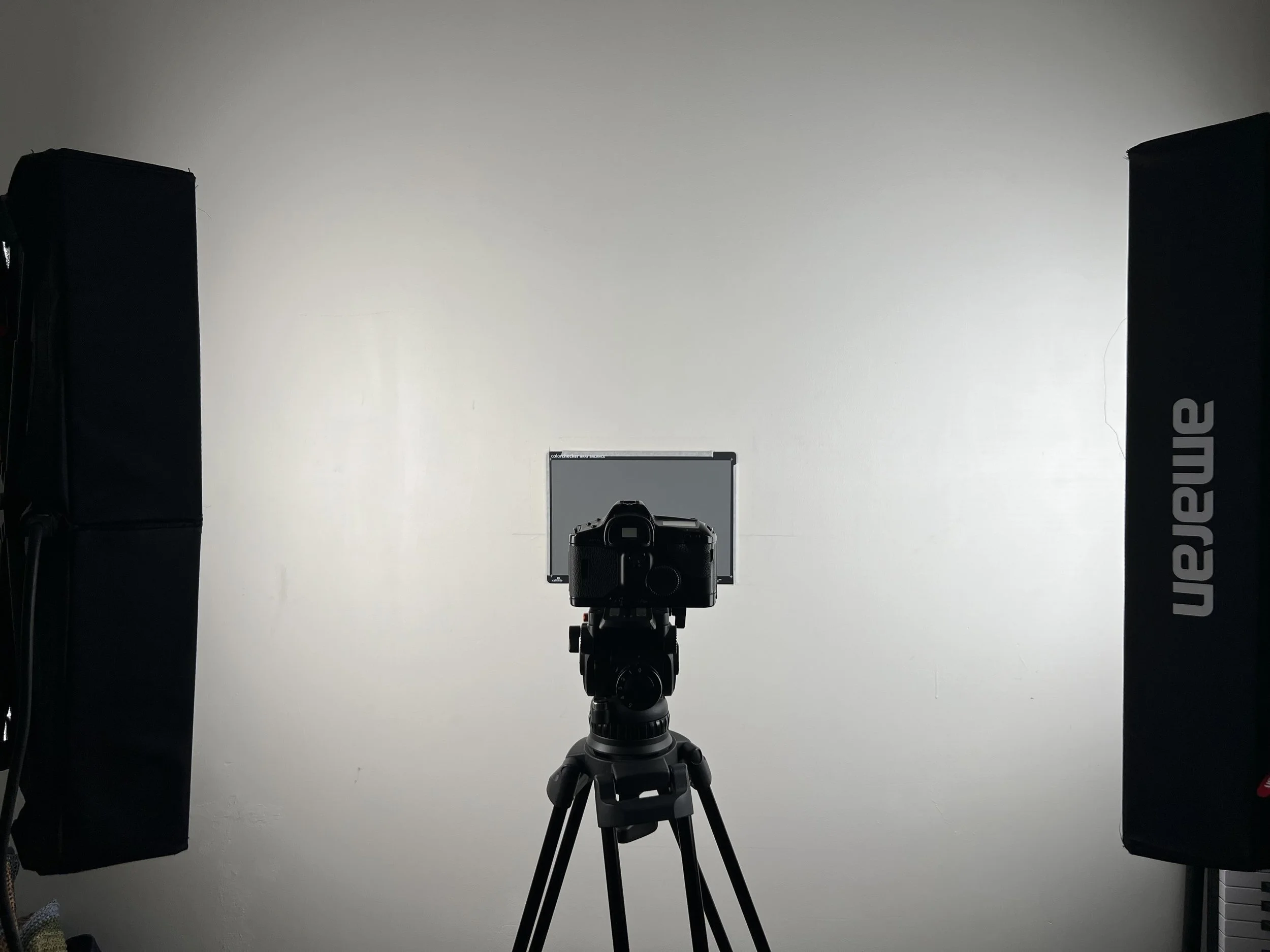
After reading about Livegrain workflow I was set to mimic their process to the letter. But I quickly realized there was a downside…it’s pretty pricey. To pull it off, you’d need to run a 35mm camera motion picture (expensive to rent) at different exposures for around 30 seconds per grain asset (around 5 to 10 exposures depending on how granular you want to be) and that’s a lot of film. Well, I wasn’t ready to spend that amount of money without even being sure it would have looked better than other readily available options. But then I realized that I could do something a little different without sacrificing authenticity. The real grain could be analyzed mathematically to understand the distribution of the grains within frame and then with those statistics figured out it would be possible to reproduce as many grain frames as needed to create a grain assets. Since the analysis is done on a single frame the whole process becomes much more budget friendly as we can create assets for the whole exposure range by shooting less then dozen frames with a still camera. The grain frames are shot by lighting a grey chart evenly. I chose to have the following exposure steps: 0EV, +2EV, +4EV, +5EV, -2EV, -4EV, -5EV. One could choose to be more granular then this but I don’t think it’s going to yield better results. I think shooting 0EV, +3EV, +5EV, -3EV, -5EV would already be enough especially when placing the grain under the S-curve of the viewing LUT.
We would then scan the grain at the highest resolution possible on our scanner or using a DSLR set up. If you followed my Scanning class I would suggest not to use the 3 (R,G,B) exposures method as taking 3 individual pictures might result in some misalignment that we definitely want to avoid in this case. (plus we’re not very much interested in color accuracy anyways). In my case I used Vuescan at the highest 7200 DPI setting, set to output a .dng raw file which is going to be quite big (468 mb per frame), but it’s quite important to make sure we capture the highest amount of detail the scanner can provide. In the process make you sure you dust off you negatives as best as you can. A few dust spots here and there aren’t much of a problem, but if there is too much dust, it would influence the statistical analysis of the grain.

Once we have our scans we can open them in Fusion Studio, debayer them to Black Magic Design Color space/linear gamma, and invert them using the cineon inversion DCTL. At this point we have to take that enormous scans crop them to 16:9 and downsample to 4K. The film area of my scans was roughly 9800×6700 8 perfs. We can crop that to 16:9 obtaining 9792×5508 and then downsample to 4K (3840:2160). It’s important to first crop and then downsample to achieve the correct appearance of the grain as if it was a native 4K scan. We can then export the frames as 16 bits tiffs no compression.

Before we start the analysis we need to turn each frame into a “zero mean” frame centered around middle grey. Right now the frames have not only different grain levels but also different brightness values. We first need to equalize those differences in exposure so that the only thing we are left with is the grain differences. To do that we can use a python script that you can find it here. Once we have the mid grey centered zero mean grain frames, we can start the grain analysis and grain generation using another python script in google colab. You can download the python script here. The script needs to run in colab as we need to use GPU acceleration as generating the grain frames on CPU locally would take a huge amount of time. Basically what the algorithm does is analyze the grain frame and output as many frames as you want with the same statistical distribution. By repeating the generation process for each exposure level we can then create the grain assets that we can composite onto the image for each exposure level. I normally generate 700 frames for each exposure which gives a grain asset of around 30 seconds. To create the grain asset we need to import all the 700 frames in resolve, and render a 4K ProRess 422 HQ video. After having repeated the process for each exposure level we can import those assets in a project as mattes and composite them onto the image in their respective luminance range.
Compositing the grain layers.
These assets are mid grey centered zero mean plates. The composite mode to use is Linear Light at .500 opacity. There is no guess work on how much strength or opacity you should use. (if you want to match the behavior of your scanned grain). Linear Light composite mode interprets 0.5 (mid grey) as no change as it subtracts it from the image, our grain plates are centered around middle grey but the amplitude of the grain creates variations both in upward and downward direction. Linear Light interprets deviations from 0.5 as double strength. So if the plate “add +0.1 brightness,” Linear Light tries to add +0.2 instead.
If it “subtract –0.1,” Linear Light subtracts –0.2.
That’s why, if you leave the blend layer at 100% opacity, everything comes out too strong.
To fix that, we set opacity to 50%. This halves the effect and brings it back to the correct level — exactly matching what your plate was designed for and affect the image with the intended amplitude.
Every grain asset gets composited onto the image in they’re respective luminance range. It doesn’t matter which log encoding you’re using. You know to which exposure level each assets corresponds to, then you simply take the luminance range of the log encoding you’re using and composite the assets onto it. We are basically masking the log image per luminance and composite the corresponding. You can download the node tree or follow the video part of the lesson to understand this more clearly.
If the grain layers are from a negative stock it’s a good idea to have them composited onto the image before the viewing LUT/S-curve. This way the grain will behave like real film, more present in the midtones, Less present in highlights and shadows because of the Scurve. If you want to have the grain at the end of the chain it could be a good idea to synthesize the grain of a print or slide film, which is already ready for display.
The last thing to keep in mind when composting a grain layer onto an image is the softness of the grain. Luckily with the Film Grain Rendering Algorithm we can decide how soft we want the grain to be therefore we know how much to soften the image before composing the grain onto it. It’s important for the image not to be sharper than the grain itself as that would produce non organic looking texture. To soften the image I like using a DCTL from Thatcher Freeman called “separable gaussian blur”, which allows us to match the same softness of the generated grain. More about this in the video section.
Here you can download the tools to generate the grain assets.
Link to Thatcher freeman tools: here you can find the DCTL interpreter to use DCTLs in the Fusion Studio as well as the Separable Gaussian Blur dctl which you’re going to see in the video.
Down below a the video section of the class covering the steps we talked about: