This is where it all starts. The data gathering. This step is crucial and if we don’t collect the data accurately in this first step the whole process is gonna suffer down line. And even if shooting charts with the 2 cameras to compare to each other might seam trivial there are many subtleties to this process that if not taken into consideration might lead to less then optimal data collection results. We need 2 cameras, a digital camera and a film camera. Film camera wise, even if you want to profile motion picture film, you can use a still camera since we’re not interest in the motion and all we need is one frame of every exposure. I highly recommend to carefully choose the film camera you’re going to use for the job as many popular and trendy film cameras on the market are not suited for high precision work.

You’re gonna need a precise and consistent shutter speed but unfortunately many film cameras have a very wide tolerance when it comes to those speeds up to more then 30% fluctuations and different fluctuations at different speeds. That would severely affect your data set accuracy. You’ll need a film camera which has an electronically controlled shutter speed. I personally use a Canon Eos1n, which gets periodically checked to unsure optimal operations, and the shutter speeds are just spot on. That being said, you’re always going to see some fluctuations if you take multiple exposure with identical settings. It has to do with still camera tolerances (even the most accurate stills film camera will have some fluctuations), There is nothing you can do about it, but don’t worry about it too much as the method of profiling that I’m going to show you in the next classes is pretty robust to those fluctuations.

THE CHARTS

Shooting Color Charts (Creating the Dataset)

If you don’t to go through the trouble of shooting your own charts but you want to start practicing with the tools and techniques you’ll learn in these classes you can download film and digital charts that I shot over here and the tools I use for the profiling over here

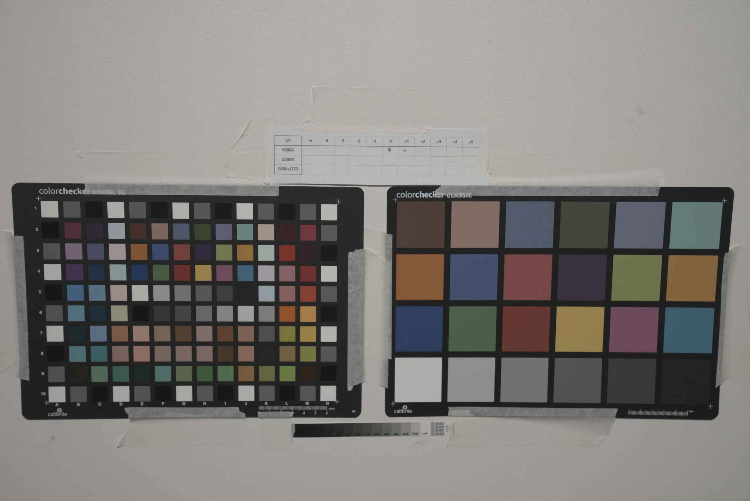
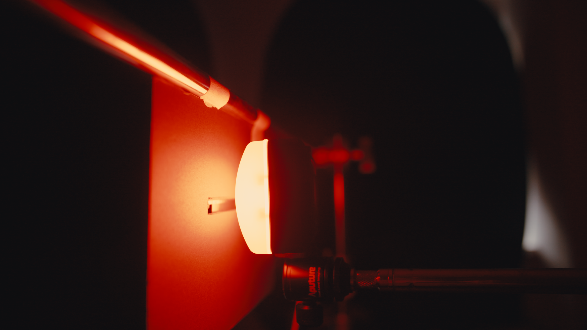
In order to create a profile of a film stock we need to gather a decent amount of data covering the whole exposure range and a rich set of colors. The best way to go about is to use charts. More specifically I’m a fan of the Color Checker Classic in combination with the color checker SG (the latter provides a  wider coverage and wider gamut colors). When one wants to build an even more solid dataset reflective charts alone are not enough, some emissive charts or sources should be added in order to capture the most saturated colors. The next thing we need is a high quality tunable light source. I would suggest using something like an Arri Orbiter which is the light I used when creating my dataset. The reality is that any professional light with a high enough SSI score will do the job. The one thing you want to look for is heat related LED output drift. LEDs tend to shift in color temperature and decrease in light output when they heat up. For this reason, choose a light source with good heat management (COB point source lights with fans are usually better compared to LED panels) The Arri orbiter didn’t shift the slightest during the testing but so did the SmallRig RC 350B.

The concept is simple you want to expose the charts to light and record them with both the digital sensor and the film stock at different exposures making sure the 2 instruments see the same exact scene (illuminated charts).

To make sure to gather a lot of data it’s important to use at least 3 illuminants.

If the film stock we’re profiling is daylight balanced we’re gonna shoot the charts at 5600k, 3200k and for the cooler color temperature I would keep the LED fixture at 5600 and use a CTB gel. (I prefer using a CTB gel rather than cranking the color temperature up to 15000 kelvin)

If the film stock is tungsten balanced we would have 3200k, 3200K + CTO gel, and 5600K

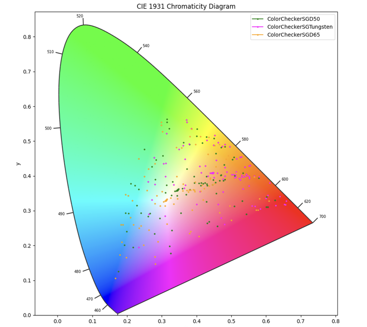
Since a color stimuli is the product of the spectral reflectance of an object and the spectral power distribution of the light hitting it, using multiple illuminants to create a dataset is the exact same thing as having a different set of patches. This way we can create a satisfying dataset without needing a chart with a huge amount of colors, we just need to capture it under different illuminants.

As you can see by changing the illuminant used to light the color chart (in this case the Color Checker SG) we change the color stimulus obtained. Therefore changing the illuminant is comparable to have a color chart with a different set of patches

Setting the Exposure

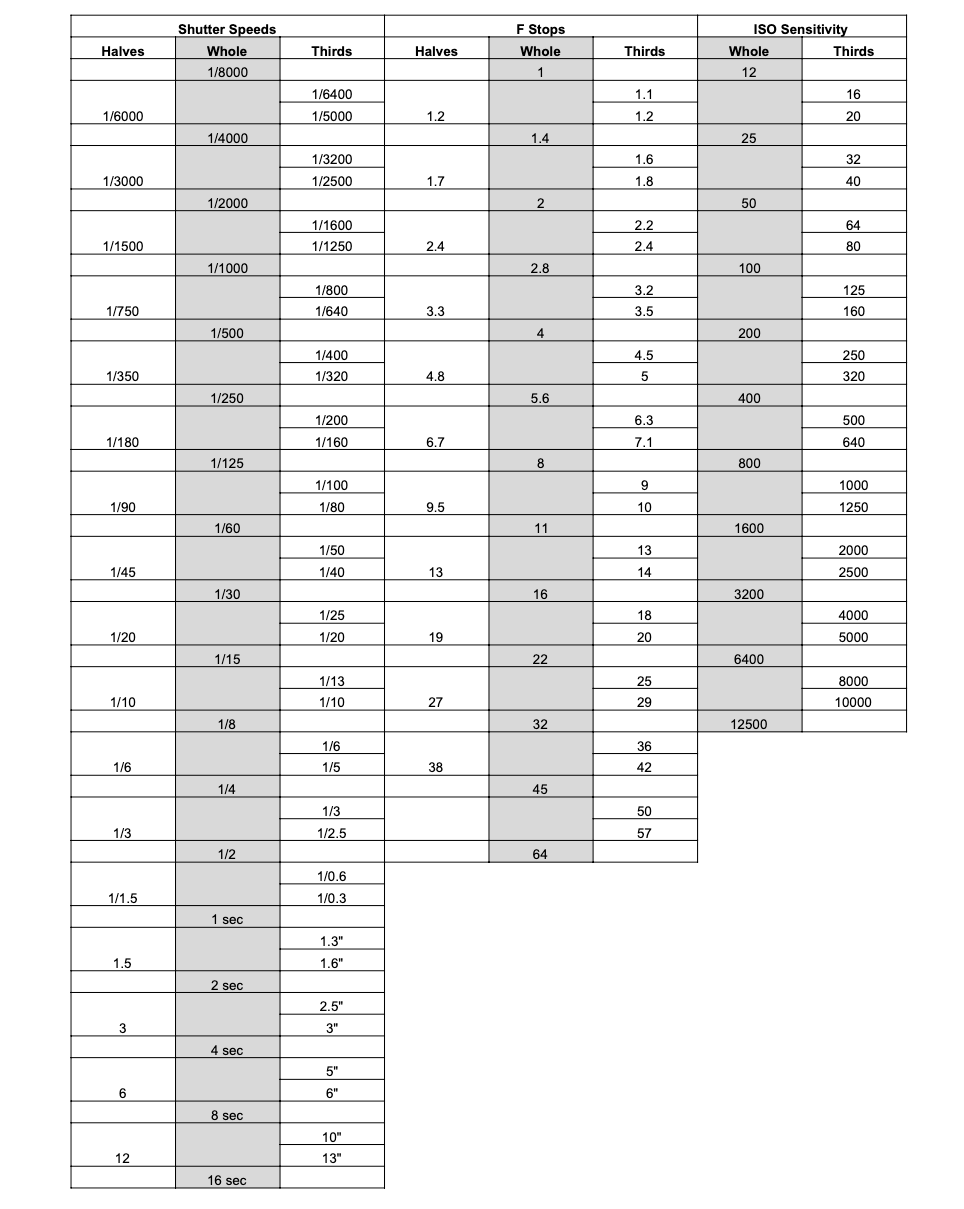
When shooting the charts It’s also important to use the same lens on both cameras in order to not introduce inconsistencies. (even if you have 2 of the same lens, it’s best to shoot the charts with camera A, then mount the same lens on camera B and repeat the process) In order to go up and down the exposure range we’re going to use the shutter speed/shutter angle and cover the whole range from 0EV to +5Ev to -5Ev in steps of 1 stop. The difference in speed (light sensitivity) between the film stock and the digital camera should be compensated with the shutter/shutter angle. If the film stock is iso 200 and the digital camera native iso is 800, in order for them to match the shutter speed on the digital camera should be set 2 stops faster (less light) than the the film stock.

Some practical examples

Using the table

Film stock iso 200, Shutter speed 1/40, F stop 5.6. //// Digital camera iso 800, Shutter speed 1/160 (twice as fast. Half the light enters. compensates for the digital camera being twice as sensitive)

Film stock iso 500, Shutter speed 1/40, F stop 5.6 //// Digital iso 800, Shutter Speed 1/60, Stop 5.6

Film iso 250, Shutter speed 1/40, Stop 5.6 //// Digital iso 800, Shutter Speed 1/125, Stop 5.6

We’re gonna see how the linearity of a digital sensor comes in handy later on. For a digital camera you could just take 1 single exposure per color temperature which as long as it’s not clipped gives you all the other exposures by simply using linear gains in post. We’ll go into details later.

To go up and down the exposure we’ll use the shutter speed and for the lowest and highest exposures if your camera doesn’t allow you to tweak shutter speeds or the film camera is been tested and it’s a little less precise at very fast shutter speeds then I normally use the aperture of the lens (only if it’s a photo lens, as cinema lenses have de-clicked apertures and makes it difficult to repeat the same exact setting)

NB. If an increase or decrease in exposure is achieved with the aperture on one camera, it should be mirrored on the other camera as well. Reference the 2 tables down below:

You might have noticed that I start the film camera at 1/40 every time. And it’s because this gives you the widest range of exact stop increments and decrements. On the digital camera this doesn’t really matter as you can probably set the shutter speed/angle at whatever speed you need. But for the film camera not all increments and decrements are exactly 1 stop. Look for exact halving and doubling of the shutter speed on your camera.

Going from 1/40 to 1/20 = 1exact stop,

from 1/20 to 1/10= 1 exact stop,

from 1/10 to 1/5 = 1 exact stop.

going from 1/125 to 1/60 is not exactly one stop.

From 1/60 to 1/30 is exactly one stop, 1/30 to 1/15 is exactly one stop, but 1/15 to 1/8 is not.

My suggestion is therefore to always have the film stock at a shutter speed of 1/40 for the 0EV chart.

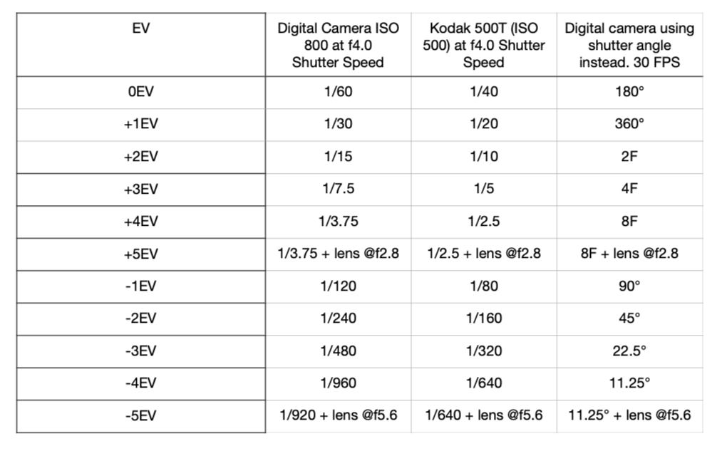
Below is an example table when shooting digital native ISO 800 and film speed ISO 500. I included the shutter speed adjustment through shutter angle as it allows for more precise adjustment. The speeds are equivalent

High purity colors datasets

As mentioned before, it’s critical to include some highly saturated colors to the dataset. Here’s the difference between 2 profiles: one made with reflective charts only, the other one by including high saturation colors in the dataset.

In order to include these high saturation colors you have different ways to go about it, but in any case you’re gonna have to switch from reflective to emissive.

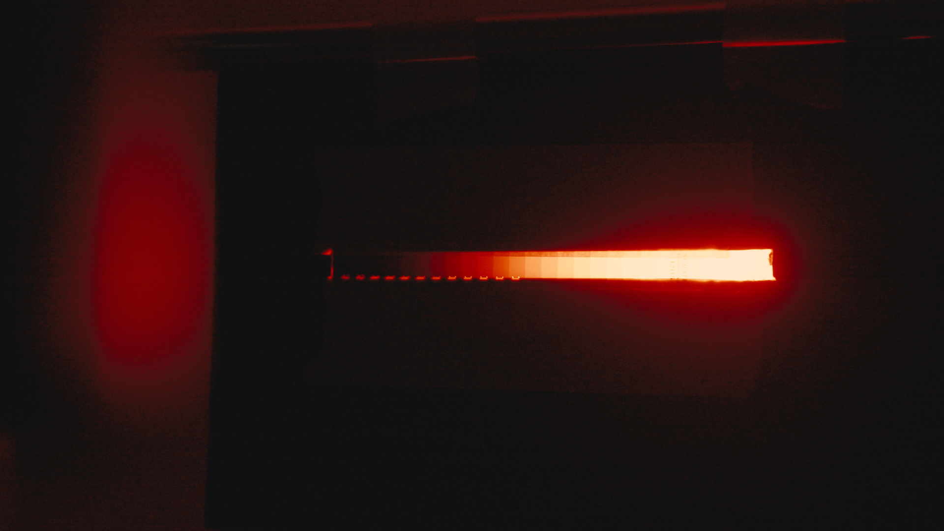
I experimented with different approaches like printing a color chart on duratrans (backlit film) but still, even the most saturated patches, weren’t saturated enough. So far my favorite method is to use a small LED light like an Aputure MC pro or Astera Hydra panel to back light a transmissive step wedge.

The advantage of such set up is that it allows to capture all the dynamic range you need in a single exposure as this step wedge covers 10.5 stops. The step wedge I’m using is the STOUFFER Stouffer Transmission Step Wedge Gray Scale #T2115. I suggest dividing the high saturation colors in RGBCMY regions and choose 6 different colors within each region. If you use a fixture like an MC pro or a Hydra panel you could directly input the xy coordinates to gather the data that you need.

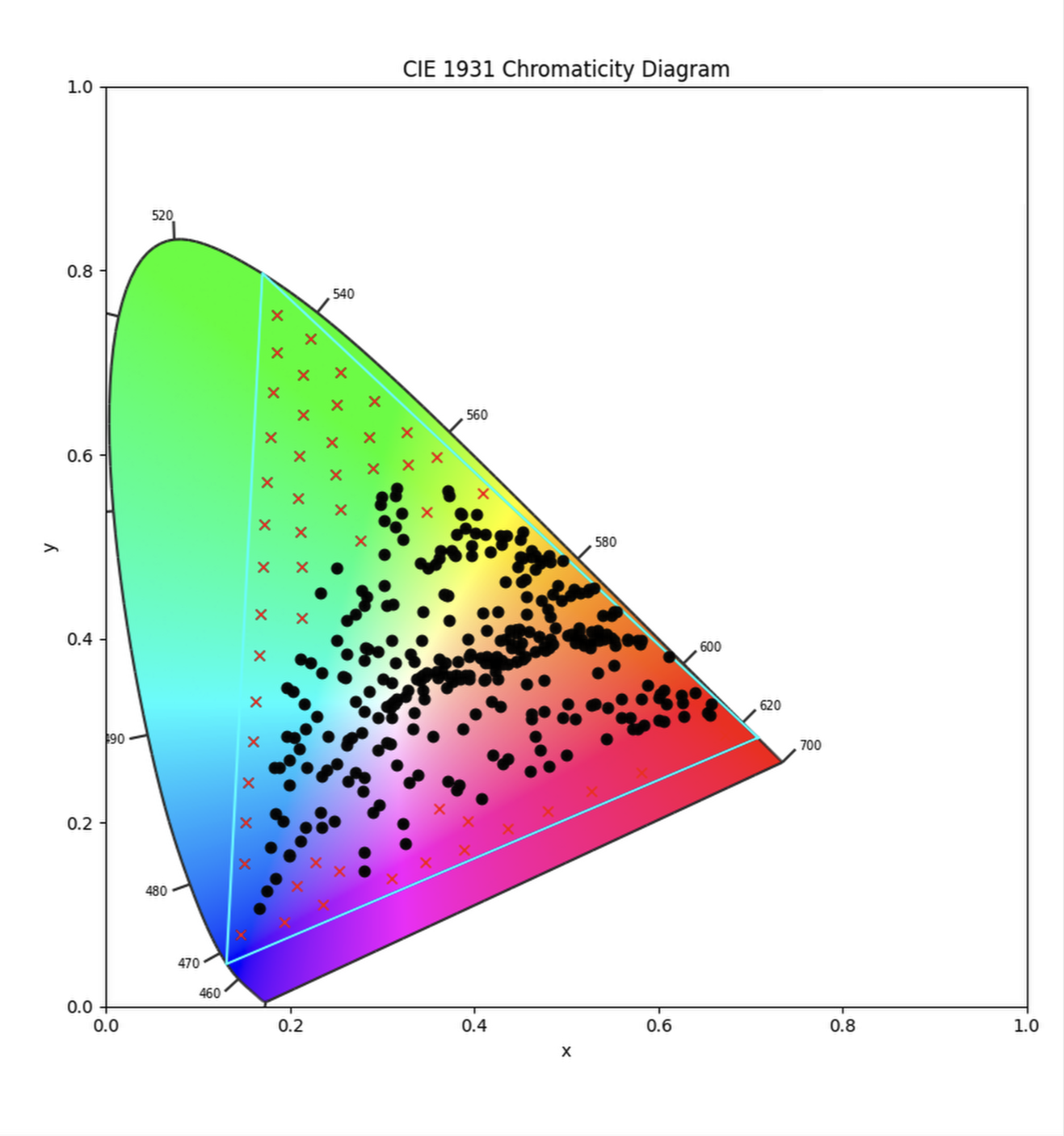
The X’s are the coordinates to fill the rec2020 color space to reach where the reflective charts can’t. I didn’t use all of the coordinates of the X’s in this graph. The important thing is to have good coverage, especially at within the highest saturation regions, but you don’t need to have such a crowded dataset. In fact I sticked to around 36 coordinates. These are coordinates you could use. But feel free to do your own testing with a spectrometer

x, y

Digital Sensors Linearity

Now let’s take a look at why I previously said that for a digital camera all you really need is 1 exposure and from there you can just compute all the other exposures in linear light in post.

Digital sensor are very linear in their response. Below is the color chart at 0Ev and the color chart at +2 EV. If we gain the the 0EV chart up of exactly 2 stops in linear we can see that the 2 images look practically identical, (not similar, identical) the only thing that changes is the noise floor, the color data remains exactly the same. You can clearly see this in the waveform if you try this experiment yourself.

0.23,0.61

0.28,0.62

0.17,0.5

0.23,0.55

0.23,0.51

0.17,0.43

0.22,0.42

0.16,0.36

0.16,0.31

0.15,0.26

0.15,0.22

0.15,0.16

0.15,0.12

0.14,0.06

0.2,0.09

0.23,0.15

0.26,0.12

0.31,0.14

This tells us that we could just gain up or down the signal and recreate the same dataset on the digital camera, plus minus the noise. in fact if you want to be noise free you could expose at plus 3 EV, making sure nothing is clipped, this will allow you to gain up 2 stops for the +5 ev without much noise increase and down to -5Ev in a very clean way. If you argue that noise is part of the image and therefore want to take it into account then you could just go through the usual up and down in 1 stop increments approach as discussed earlier.